 GitHub
 YouTube
Motor Control University
Embedded code implementation - Real-time
Discrete time execution
Simulations are typically performed in the continuous time domain using Matlab/Simulink :registered:. A differential equation solver is used to solve simulation outputs. The real-time embedded software does not implement such solver so a discrete-time equivalent controller must be used. In the model, the continuous time integrator or transfer functions needs to be replaced by discrete time equivalent. Depending on sampling time, the controller synthesis may require special attention. Here it is assumed that sampling frequency is higher enough than system bandwidth, to keep continuous controller synthesis. The dynamic controller synthesis is described in the controller page.
Scheduler
Matlab/Simulink enables multi-rate model with blocs executions at different sampling frequency. For each block, it is possible to set its rate and its offset. Blocks rate offset are multiple of the base model time step defined in the solver panel. A multi-rate model can be implemented using a multi-tasking scheduler (default settings) or a single tasking program.
Single tasking program
In a Single tasking program, all tasks started at a given base model time step must be completed within the end of that time step slot to respect real-time constraints. The fastest task, as well as all other tasks, starting at a given period must be completed before the end of this period in order to respect real-time constraints. This is a strong constraint on the slowest tasks, which may need to be split into multiple tasks whose execution is shifted in time.
Multi tasking scheduler
In a Multi tasking scheduler, a monotonic-rate scheduler is implemented where higher rate tasks have higher priority and interrupt lower task rate which have lower priority whenever required. This multi-tasking scheduler has a simple priority rule which is well suited for automatic control. Its limited implementation penalty in execution time worth the gain in flexibility. The multi-tasking rate monotonic scheduler principle is illustrated on the figure below.
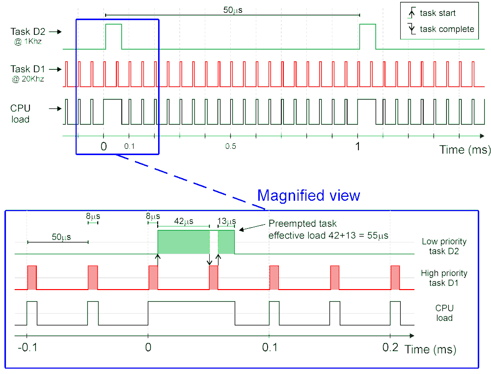
The figure presents a timing analysis for a motor control with the CPU load state (black curve where 1 is busy and 0 is idle state), the fast task D1 (red) and slow task D2 (green) respective start and stop on rising and falling edges.
The lower graph is a magnification of the higher priority task D1 preemption of the lower priority task D2. Note that, the slow D2 task is not cleared when being preempted but exclusively when task is completed. The shaded region in the tasks D1 and D2 shows the CPU execution on each task. This illustrates the benefit of a Multi-tasking scheduler as presented on the Figure.
Simulink highlights blocks with colors to represent rates as represented on the figure. This option is displayed by clicking on the “Sampling Time” icon represented by two blue and red arrows.
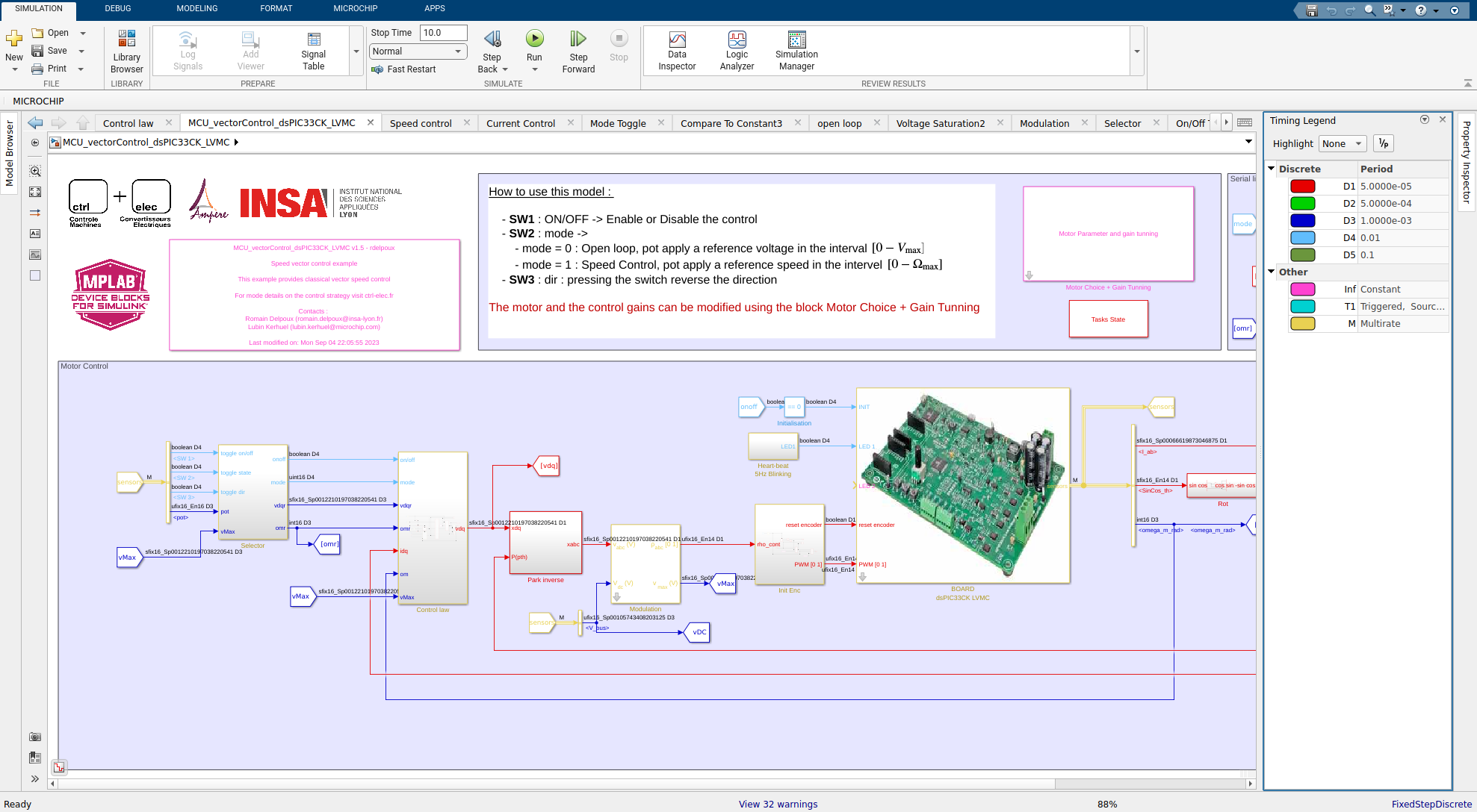
The timing legend obtained on the Simulink model for the vector control example (download from git) highlight 5 discrete time tasks :
- D1 (red) - period of \(5\times10^{-5}\)s (\(20\)kHz), is the fastest task. It computes the current measurements, Clarke and Park transformations, the electrical dynamic control, the voltage saturation management, the modulation (Sine or SVM) and update the duty cycle, send to the PWM peripheral. The task has the highest priority and requires particular care when programming to avoid overloading the CPU.
- D2 (green) - period \(5\times10^{-4}\)s (\(2\)kHz) is dedicated to the data visualization. Data to be monitored in real time are send through UART protocol and can be visualize on a computer using data visualization tool (picgui).
- D3 (blue) - period \(1\times10^{-3}\)s (\(1\)kHz) computes the speed measurement and the outer control law (mechanical control), which require a smaller bandwidth insofar as the dynamics are slower.
- D4 (light blue) - period \(1\times10^{-2}\)s (\(100\)Hz) treats the on-board switches used to change the control modes on the example.
- D5 (dark green) - period \(1\times10^{-1}\)s (\(10\)Hz) blinks the Heart-Beat led (5Hz). This visual test ensures that the DSC is operating correctly.
Code efficiency
The code performance are surprisignly good. Peripheral are handled as in background through interrupts. Peripheral blocks for input peripherals are thus not blocking as they just have to read the last result obtained from that peripheral; keeping the CPU time dedicated to the control algorithm. For example, the base time step is typically triggered by the ADC block end of conversion interrupt thus when the ADC block is evaluated within the algorithm, the conversion results are already available. The ADC block do not have to wait for a sample and hold sequence nor by the following conversion sequence. The same remark holds for others peripheral blocks like the UART transmission/reception, the SPI or I2C blocks …
Code replacement
This MathWorks functionality allows replacing code of standard Simulink blocks by an optimized code for the target so as to benefit from the optimized target hardware architecture like its DSP unit or specific instruction set. Code replacement is implemented for common operations like rounding, saturation and few operations on matrix. It is also implemented for functions like square root, sine and cosine functions when used with fixed point data type input.
Temporal analysis tools
Some blocks are available for timing analysis. #### CPU (Central Processing Unit) overload
The block detects overload. A physical pin can be used to detect an overload through a LED or a scope. A block output can provide overload information to the embedded program. The pin output works asynchronously: the pin is set as soon as an overload occurs and is never reset by the DSC (Digital Signal Controller) load block. It is however possible to reset the pin using a “digital output write” block which can be set again by the CPU overload block. The block output works synchronously. For each CPU overload block present on the model, any overload occurrence between successive evaluation of the block are reported in a 16 bit-field integer where the bit 0 code for an overload of the task D0 (fastest rate), bit 1 for the task D1 until D14. The bit D15 represents overload on task D15 and higher if the model use more than 16 different tasks.
CPU load
The block measures the overall load of the DSCs. It can output the load by toggling a pin. The high state shows the load. The block can also measures the DSC load using internal timers providing the value to the embedded program as a block output. A timer is incremented when the DSC is either running a task, or running a peripheral interrupt (i.e. not idle). The block report the timer increment between two evaluations of this block. The timer resolution should be selected to be able to measure a period corresponding to the block sample time. The measured time should be equal or lower than the block sample time. It’s worth noticing that a \(100\%\) load on one time step (for example in monotonic scheduler figure from time \(0\) to $50$s) does not mean that an overload takes place.
Multiple CPU load blocks can be placed within one model with different sample times, allowing to average the load over different time period corresponding to the respective block sample time.
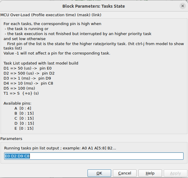
Task State
The block allows the representation of the tasks execution state through output pin. Each pin representing one selected task. Each task switches its pin high when it starts, and switches back its dedicated pin low when completed. For the proposed vector control example (download from git), the tasks are affected as follow
- tasks D1 is affected to pin E0 can be visualized on the board thanks to mikroBUS B connector, pin AN
- tasks D2 is affected to pin D2 can be visualized on the board thanks to mikroBUS B connector, pin RST
- tasks D3 is affected to pin D9 can be visualized on the board thanks to mikroBUS B connector, pin CS
- tasks D4 is affected to pin C8 can be visualized on the board thanks to mikroBUS B connector, pin SCK
A screenshot of the task state configuration window is shown below:
The tasks states execution was recorded with an oscilloscope and the result is given below:

The figure highlight that the fastest task D1, with sampling time at \(50\)us, takes only \(13\)us to perform all your calculations (26% of the load only), while this critical high speed task realizes tedious calculations (Clarke and Park transformations, electrical dynamic control, modulation (Sine or SVM), voltage saturation management, …). This leaves 74% of the load to add more advanced algorithms (state observers, parameter identification).
Task D2 is dedicated to data transfer for visualization (see page Data Visu).
Task D3 is dedicated to the mechanical dynamic control. 38% of the load at this rate is still available. D3 task, with sampling time at \(1\times10^{-3}\)s, uses \(15\)us which represents only \(1.5\%\) of the load at this rate.
The figure also illustrates the monotonic-rate scheduler and the succession of tasks with decreasing priorities.

