 GitHub
 YouTube
Motor Control University
Embedded controller optimization
This section describes some of the work obtained as part of Hiba Houmsi’s thesis work, in collaboration with Federico Bribiesca Argomedo, Paolo Massioni and Romain Delpoux. These results have been published in (Houmsi2023_VPPC). A solution to embed optimal control methods based on convex optimization directly into microcontrollers is described. A simple, targeted, LMI (Linear Matrix Inequality) solver has been developed for this scope (Massioni2024).
In the section FOC - Control a classical cascaded vector control, based on the motor frequency separation (i.e. a fast electrical dynamics and a slower mechanical dynamics) was proposed. The separation principle allows the design of two separate controllers with second order dynamics which allow to find the controllers gains easily using pole placement methods (Ackerman’s formula). In more complicated cases controller gain tuning is a non-trivial task, where the user is required to set a specific value for the poles or the cost functions, rather than an acceptable range of values. The robust pole placement LMIs regions method presented in (Chilali1999) is very interesting in this perspective, as it allows one to just set an acceptable desired region of the complex plane for the closed loop poles.
Electric motor model
Using Clarke and Park’s transformations the PMSM mathematical model in the d-q frame is expressed as: \[ \begin{equation} \begin{cases} L\frac{di_d}{dt} = v_d - Ri_d +pL\omega i_q, \\ L\frac{di_q}{dt} = v_q -Ri_q -pL\omega i_d - p \phi_f\omega, \\ J\frac{d\omega}{dt} = \frac{3}{2}p\phi_fi_q -f\omega -\tau_l; \end{cases} \label{eq:modelnonlineaire} \end{equation} \]
where the inputs of the system are \(v_d\), \(v_q\), the d-q phase voltages and the measured states of the system are \(i_d\), \(i_q\) and \(\omega\) respectively the d-q phase currents and rotor angular speed, \(R\) the phase resistance, \(L\) the phase inductance, \(\phi_f\) the peak magnetic flux of the permanent magnets seen by stator windings, \(p\) the pole pairs number, \(J\) the inertia of the system, \(f\) is the viscous frictional coefficient of the motor, \(\tau_l\) the load torque considered as an exogenous disturbance (not measured). The system described previously is nonlinear due to the product of two state variables, so a feedback linearization method is applied (Bodson1993) to eliminate these nonlinear terms. Choosing: \[ \begin{cases} v_d = u_d-pL\omega i_q,\\ v_q = u_q +pL\omega i_d, \end{cases} \] the system can be then rewritten as: \[ \left\{\begin{array}{lcl} L\frac{di_d}{dt} &=& u_d - Ri_d,\\ L\frac{di_q}{dt} &=& u_q - Ri_q - p \phi_f\omega,\\ J\frac{d\omega}{dt} &=& \frac{3}{2}p\phi_fi_q -f\omega -\tau_l. \end{array}\right. \] One can split this system into two independent linear time-invariant systems: a first-order system that characterizes \(i_d\) dynamic, and a second-order system that describes \(i_q\) and \(\omega\) dynamics. A controller is built for each subsystem and, to ensure zero steady state error in the presence of constant disturbances and parameter mismatch, the state space model is augmented with an integral action. The tracking error can be defined as: \[ \begin{equation} %\begin{multlined} \dot{e}_i = \begin{bmatrix} -\frac{R}{L} & 0\\ 1 & 0 \end{bmatrix} e_i + \begin{bmatrix} \frac{1}{L} \\ 0 \end{bmatrix} u_d %\end{multlined} \label{eq:dynamiqueid} \end{equation} \] where \(e_i=\begin{bmatrix}i_d- i_{d}^\#&\varepsilon_i\end{bmatrix}\) and \(\varepsilon_i=\int_0^t(i_d - i_{d}^\#)dt\) the integral action over the output of the system \(\varepsilon_i\). The tracking error state space model of the \(i_q\) and \(\omega\) dynamic: \[ \begin{equation} \dot{e}_{\omega} = \begin{bmatrix} -\frac{R}{L} & \frac{p\phi_f}{L} & 0\\ \frac{3p\phi_f}{2J} & \frac{-f}{J} & 0 \\ 0 & -1 & 0 \end{bmatrix}e_{\omega} + \begin{bmatrix} \frac{1}{L}\\ 0 \\ 0 \end{bmatrix} u_q \label{eq:dynamiqueOmega} \end{equation} \] where \(e_\omega=\begin{bmatrix}i_q&\omega-\omega^{\#}&\varepsilon_\omega\end{bmatrix}\) and \(\varepsilon_\omega=\int_0^t(\omega-\omega^\#)dt\) the integral action over the output of the system \(\varepsilon_\omega\). Both models can be written in the classical state-space form: \[ \begin{equation} \dot{x}(t) = Ax(t)+Bu(t) \end{equation} \] with \(x\in \mathbb{R}^n\), \(u\in \mathbb{R}^m\) and with appropriate definitions of \(n,~m,~x(t),~u(t),~A\) and \(B\).
The primary objective of a control system is then to guarantee stability and performance when subject to unknown disturbances and parametric variation. Ultimately, this involves determining the state-feedback gain \(K\) for the control law: \[ \begin{equation} u(t) = Kx(t) \label{state feedback} \end{equation} \] in a way that, when such a control is applied, the closed-loop system in the following form: \[ \begin{equation} \dot{x}(t)= (A+BK)x(t) \end{equation} \] possesses the desired properties.
Regional pole placement
This subsection provides a synthesis of how a resilient pole placement via LMIs (Chilali1999) can be utilized to synthesize the full-feedback gain matrix. The goals are the following:
- the closed-loop dynamics has to be asymptotically stable (i.e., the error converges to zero),
- the closed-loop poles should guarantee an exponential decay rate \(\alpha\) within a minimum \(\alpha_{min}\) and maximum \(\alpha_{max}\) values,
- the damping factor of the system \(z\) should be greater than a minimum specified value \(z \geqslant \frac{1}{\sqrt{1+\beta^2}}\) expressed in terms of a positive tuning parameter \(\beta\).
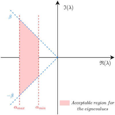
The figure depicts the constraints \(\alpha_{min}\), \(\alpha_{max}\) and \(\beta\) over the real and imaginary parts of the eigenvalues of the closed-loop system.
Finding a controller gain matrix \(K\) that satisfies these specifications boils down to the following LMI feasibility problem: \[ \begin{array}{l} \underset{x}{\mathrm{find}} \ L \in \mathbb{R}^{m \times n},\, X=X^\top \in \mathbb{R}^{n \times n} \ \mathrm{s.t.} \\ \begin{array}{l} H_1 &=& X \succ 0\\ H_2 &=& -\left(XA^\top+L^\top B^\top + AX+BL +2X\alpha_{min}\right)\succ 0 \\ H_3&=& XA^\top+L^\top B^\top + AX+BL +2X\alpha_{max}\succ 0 \\ H_4 &=& -\begin{bmatrix} \beta (XA^\top+\!L^\top B^\top+AX+BL ) & AX+BL-XA^\top-\!L^\top B^\top\\ XA^\top+\!L^\top B^\top-AX-BL & \beta (XA^\top+L^\top B^\top+AX+BL) \end{bmatrix} \succ 0 \end{array} \end{array} \] With an affine parameterization of \(X\), \(L\) as \(X(\xi)\), \(L(\xi)\) where \(\xi \in \mathbb{R}^{\mu}\), is a vector of decision variables, with \(\mu=\frac{n(n+1)}{2}+n\times m\). This problem can be solved with standard semidefinite programming constrained optimization methods, and the controller can then be retrieved with the transformation \[K=L X^{-1}.\]
Notice that the existence of a solution for the problem above is a sufficient condition for the existence of a controller that successfully places the poles in the desired area, but not necessary. This is due to the conservatism involved in the convexification of the problem, see again (Chilali1999) for details.
To solve such an optimization problem, SeDuMi solver (Sturm1999) and Yalmip parser (Löfberg2004) can be used. To illustrate, on the a PMSM motor example, the off-line solution of the optimization problem, a Matlab LiveScript is proposed on GitHub : regionalPolePlacement_Yalmip.mlx.
Interior point solver
The optimization problem in this case is a feasibility problem which can be solved by means of an interior point algorithm, whose working principle is based on turning the constrained optimization into an unconstrained one, on which Newton iterations can be applied (Vandenberghe1997) . This conversion is obtained through the use of an augmented cost function that includes a barrier function, i.e., a term going to infinity when the edge of the constrained region is approached.
The problem can be put in a single inequality as: \[ \begin{equation} F = \begin{bmatrix} H_1 & 0 & 0 & 0 \\ 0 & H_2 & 0 & 0 \\ 0 & 0 & H_3 & 0 \\ 0 & 0 & 0 & H_4 \end{bmatrix}\succ 0 \end{equation} \] where \(F\) is a symmetric matrix affine in the unknowns \(\xi\), i.e.: \[ \begin{equation} F(\xi)=F_0+\sum_{i=1}^{\mu}\xi_i F_i \end{equation} \] where \(F_i\) are constant, symmetric matrices. The problem is then equivalent to finding a value \(\xi^\star\) of \(\xi\), for which \(F(\xi^\star) \succ 0,\) which is also equivalent to finding values \(\xi^\ast\), \(\lambda^\ast<0\) for which : \[ \begin{equation}F(\xi^\ast) + \lambda^\ast I \succ 0.\label{eq:flambda}\end{equation} \] Notice that for the problem in this last formulation, it is always possible to find a simple feasible starting point (a set of \(\xi\), \(\lambda\) for which the inequality is satisfied) by simply taking \(\xi=0\), and \(\lambda > -\underline{\lambda}(F_0)\), with \(\underline{\lambda}(F_0)\) the minimum eigenvalue of \(F_0\). The interior point algorithm that we use is summarized here.
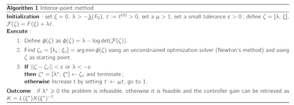
Algorithm can be found in (Boyd2004) page 569 algorithm 11.1
The barrier term in this algorithm is minus the logarithm of the determinant of \(\mathcal{F}\), which goes to plus infinity if one of the eigenvalues of \(\mathcal{F}\) goes to zero, assuring that the algorithm never exits the \(\mathcal{F}(\zeta)\succ 0\) zone as it is initialized inside it.
To solve this problem, a simple, targeted, LMI (Linear Matrix Inequality) solver has been developed for this scope (Massioni2024) initially for Arduino, and adapted for Matlab/Simulink. The same problem as the one proposed above with SeDuMI and Yalmip is solved offline with the embedded solver and a Matlab LiveScript is proposed on GitHub : regionalPolePlacement_EmbSolver.mlx.
Simulink model
An example for the real time implementation can be downloaded and tested by following the instruction on GitHub
References
(Bodson1993) Bodson, M., Chiasson, J.-N., Novotnak, R.-T., & Rekowski, R.-B. (1993). High performance nonlinear feedback control of a permanent magnet stepper motor. IEEE Transactions on Control Systems Technology, 1(1), 5–14. https://doi.org/10.1109/87.221347
(Boyd2004) S. Boyd and L. Vandenberghe, Convex optimization. Cambridge university press, 2004.
(Chilali1999) M. Chilali, P. Gahinet and P. Apkarian, “Robust pole placement in LMI regions,” in IEEE Transactions on Automatic Control, vol. 44, no. 12, pp. 2257-2270, Dec. 1999
(Houmsi2023_VPPC) H. Houmsi, P. Massioni, F. Bribiesca Argomedo, R. Delpoux, Embedded controller optimization for efficient electric motor drive, Proceedings of the 2023 Vehicular Power and Propulsion Conference (VPPC), October 2023, Milano, Italy.
(Löfberg2004) J. Löfberg, “Yalmip : A toolbox for modeling and optimization in matlab,” in In Proceedings of the CACSD Conference, (Taipei, Taiwan), 2004.
(Massioni2024) P. Massioni, ArduinoLMI https://github.com/pmassio/ArduinoLMI/, 2024.
(Sturm1999) J. Sturm, “Using SeDuMi 1.02, a MATLAB toolbox for optimization over symmetric cones,” Optimization Methods and Software, vol. 11–12, pp. 625–653, 1999. Version 1.05 available from http://fewcal.kub.nl/sturm.
(Vandenberghe1997) L. Vandenberghe and V. Balakrishnan, Algorithms and software for LMI problems in control,IEEE Control Systems Magazine, vol. 17, no.5, pp. 89–95, 1997.

